I’ve been lucky enough to have funding from SEPnet to create a new lecture course recently, following on from David Tong’s famous Part III course on string theory. The notes are intended for the beginning PhD student, bridging the gap between Masters level and the daunting initial encounters with academic seminars. If you’re a more experienced journeyman, I hope they’ll provide a useful reminder of certain terminology. Remember what twist is? What does a D9-brane couple to? Curious about the scattering equations? Now you can satisfy your inner quizmaster!
Here’s a link to the notes. Comments, questions and corrections are more than welcome.
Thanks are particularly due to Andy O’Bannon for his advice and support throughout the project.
This week I’m at the CERN winter school on supergravity, strings and gauge theory. Jonathan Heckman’s talks about a top-down approach to 6D SCFTs have particularly caught my eye. After all the theory is in some sense the mother of my favourite playground in four dimensions.
Unless you’re a supersymmetry expert, the notation should already look odd to you! Why do I write down two numbers to classify supersymmetries in 6D, but one suffices for 4D. The answer comes from a subtlety in the definition of the superalgebra, which isn’t often discussed outside of lengthy (and dull) textbooks. Time to set the record straight!
At kindergarten we learn that supersymmetry adds fermonic generators to the Poincare algebra yielding a “unique” extension to the possible spacetime symmetries. Of course, this hides a possible choice – there are many fermionic representations of the Lorentz algebra one could choose for the supersymmetry generators.
Folk theorem: anything you want to prove can be found in Weinberg.
Fortunately, mathematical consistency restricts you to simple options. For the algebra to close, the generators must live in the lowest dimensional representations of the Lorentz algebra – check Weinberg III for a proof. You’re still free to take many independent copies of the supersymmetry generators (up to the restrictions placed by forbidding higher spin particles, which are usually imposed).
Therefore the classification of supersymmetries allowed in different dimensions reduces to the problem of understanding the possible spinor representations. Thankfully, there are tables of these.
Reading carefully, you notice that dimensions , and are particularly special, in that they admit Majorana-Weyl spinors. Put informally, this means you can have your cake and eat it! Normally, the minimal dimension spinor representation is obtained by imposing a Majorana (reality) or Weyl (chirality) condition. But in this case, you can have both!
This means that in or , the supersymmetry generators can be chosen to be chiral. The stipulation says that should be a left-handed Majorana spinor, for instance. In a Majorana spinor must by necessity contain both left-handed and right-handed pieces, so this choice would be impossible! Or, if you like, should I choose to be a left-handed Weyl spinor, then it’s conjugate is forced to be right-handed.
I spent last week at the Perimeter Institute in Waterloo, Ontario. Undoubtedly one of the highlights was Juan Maldenena’s keynote on resolving black hole paradoxes using wormholes. Matt’s review of the talk below is well worth a read!
The cosmic microwave background (CMB) is a key observable in cosmology. Experimentalists can precisely measure the temperature of microwave radiation left over from the big bang. The data shows very small differences in temperature across the sky. It’s up to theorists to figure out why!
The most popular explanation invokes a scalar field early in the universe. Quantum fluctuations in the field are responsible for the classical temperature distribution we see today. This argument, although naively plausible, requires some serious thought for full rigour.
Talks by cosmologists often parrot the received wisdom that the two-point correlation function of the scalar field can be observed on the sky. But how exactly is this done? In this post I’ll carefully explain the winding path from theory to observation.
First off, what really is a correlation function? Given two random variables and we can (roughly speaking) determine their correlation as
Intuitively this definition makes sense – in configurations where and share the same sign there is a positive contribution to the correlation.
There’s another way of looking at correlation. You can think of it as a measure of the probability that for any random sample of there will be a value of within some given distance. Hopefully this too feels intuitive. It can be proved more rigorously using Bayes’ theorem.
This second way of viewing correlation is particularly useful in cosmology. Here the random variables are usually position dependent fields. The correlation then becomes
where the average is over the whole sky with the direction of the vector fixed. The magnitude of this vector provides a natural distance scale for the probabilistic interpretation of correlation. We see that the correlation is an avatar for the lumpiness of the distribution at a particular distance scale!
Now let’s focus on the CMB. The temperature fluctuations are defined as the percentage deviation from the average temperature at each point on the sky. Mathematically we write
where defines a point on the unit -sphere. We want to relate this to theoretical predictions. Given our discussion above, it’s not surprising that our first step is to compute the correlation function
where the average is over the whole sky with the angle between and fixed. This average doesn’t lose any physical information since there’s no preferred direction in the sky! We can conveniently encode the correlation function using spherical harmonics
The coefficients are known as the multipole moments of the temperature distribution. Substituting this in the correlation function definition we obtain
where . We’re almost finished with our derivation! The final step is to convert from the correlation function to it’s momentum space representation, known as the power spectrum. With a little work, you can show that the power at multipole number is given by
This is exactly the quantity we see plotted from sky map data on graphs comparing inflation theory to experiment!
From the theory perspective, this quantity is fairly easy to extract. We must compute the power spectrum of the primordial fluctuations of the inflation field. This is merely a matter of quantum field theory, albeit in de Sitter spacetime. Perhaps the most comprehensive account of this procedure is provided in Daniel Baumann’s notes.
Without going into any details, it’s worth mentioning a few theoretical models. The simplest option is to have a massless free inflaton field. This gives a scale-invariant power spectrum, which is almost correct! Adding mass corrects this result, providing fluctuations in the power spectrum. This is a better approximation, but has been ruled out by Planck data.
Clearly we need a more general potential. Here’s where the fun starts for cosmologists. The buzzwords are effective field theory, string inflation, non-Gaussianity and multiple fields! But that’ll have to wait for another blog post.
The simple answer is – everything! If there’s a symmetry in your theory then the associated Noether charge must be conserved at a Feynman vertex. A simple and elegant rule, and one of the great strengths of Feynman’s method.
Even better, it’s not hard to see why all charges are conserved at vertices. Remember, every vertex corresponds to an interaction term in the Lagrangian. These are automatically constructed to be Lorentz invariant so angular momentum and spin had better be conserved. Translation invariance is built in by virtue of the Lagrangian spacetime integral so momentum is conserved too.
Internal symmetries work in much the same way. Color or electric charge must be conserved at each vertex because the symmetry transformation exactly guarantees that contributions from interaction terms cancel transformations of the kinetic terms. If you ain’t convinced go and check this in any Feynman diagram!
But watch out, there’s a subtlety! Suppose we’re interested in scalar QED for instance. One diagram for pair creation and annihilation looks like
Naively you might be concerned that angular momentum and momentum can’t possibly be conserved. After all, don’t photons have spin and mass squared equal to zero? The resolution of this apparent paradox is provided by the realization that the virtual photon is off-shell. This is a theorist’s way of saying that it doesn’t obey equations of motion. Therefore the usual restrictions from symmetries do not apply to the virtual photon! Thinking another way, the photon is a manifestation of a quantum fluctuation.
Erratum: a previous version of this article erroneously claimed that Noether’s second theorem is related to Ward identities that guarantee gauge invariance at the quantum level. This is not the case, to our knowledge. Indeed, the Ward identity is a statement about averaging over field configurations, which necessarily depends on the behaviour of the path integral measure, a quantity that Noether never concerned herself with! Interestingly, there is a connection between the second theorem and large residual gauge symmetries, as pointed out in https://arxiv.org/abs/1510.07038.
All too soon we’ve reached the end of a wonderful conference. Friday morning dawned with a glimpse of perhaps the most impressive calculation of the past twelve months – Higgs production at three loops in QCD. This high precision result is vital for checking our theory against the data mountain produced by the LHC.
It was well that Professor Falko Dulat‘s presentation came at the end of the week. Indeed the astonishing computational achievement he outlined was only possible courtesy of the many mathematical techniques recently developed by the community. Falko illustrated this point rather beautifully with a word cloud.
As amplitudeologists we are blessed with a incredibly broad field. In a matter of minutes conversation can encompass hard experiment and abstract mathematics. The talks this morning were a case in point. Samuel Abreu followed up the QCD computation with research linking abstract algebra, graph theory and physics! More specifically, he introduced a Feynman diagram version of the coproduct structure often employed to describe multiple polylogs.
Dr. HuaXing Zhu got the ball rolling on the final mini-session with a topic close to my heart. As you may know I’m currently interested in soft theorems in gauge theory and gravity. HuaXing and Lance Dixon have made an important contribution in this area by computing the complete -loop leading soft factor in QCD. Maybe unsurprisingly the breakthrough comes off the back of the master integral and differential equation method which has dominated proceedings this week.
Last but by no means least we had an update from the supergravity mafia. In recent years Dr. Tristan Dennen and collaborators have discovered unexpected cancellations in supergravity theories which can’t be explained by symmetry alone. This raises the intriguing question of whether supergravity can play a role in a UV complete quantum theory of gravity.
The methods involved rely heavily on the color-kinematics story. Intriguingly Tristan suggested that the double copy connection because gauge theory and gravity could form an explanation for the miraculous results (in which roughly a billion terms combine to give zero)! The renormalizability of Yang-Mills theory could well go some way to taming gravity’s naive high energy tantrums.
There’s still some way to go before bottles of wine change hands. But it was fitting to end proceedings with an incomplete story. For all that we’ve thought hard this week, it is now that the graft really starts. I’m already looking forward to meeting in Stockholm next year. My personal challenge is to ensure that I’m among the speakers!
Particular thanks to all the organisers, and the many masters students, PhDs, postdocs and faculty members at ETH Zurich who made our stay such an enjoyable and productive one!
Note: this article was originally written on Friday 10th July.
One of the first pieces of Bach ever recorded was August Wilhelmj’s arrangement of the Orchestral Suite in D major. Today the transcription for violin and piano goes by the moniker Air on the G String. It’s an inspirational and popular work in all it’s many incarnations, not least this one featuring my favourite cellist Yo-Yo Ma.
This morning we heard the physics version of Bach’s masterpiece. Superstrings are nothing new, of course. But recently they’ve received a reboot courtesy of Dr. David Skinner among others. The ambitwistor string is an infinite tension version which only admit right-moving vibrations! At first the formalism looks a little daunting, until you realise that many calculations follow the well-trodden path of the superstring.
Now superstring amplitudes are quite difficult to compute. So hard, in fact, that Dr. Oliver Schloterrer devoted an entire talk to understanding particular functions that emerge when scattering just strings at next-to-leading order. Mercifully, the ambitwistor string is far more well-behaved. The resulting amplitudes are rather beautiful and simple. To some extent, you trade off the geometrical aesthetics of the superstring for the algebraic compactness emerging from the ambitwistor approach.
This isn’t the first time that twistors and strings have been combined to produce quantum field theory. The first attempt dates back to 2003 and work of Edward Witten (of course). Although hugely influential, Witten’s theory was esoteric to say the least! In particular nobody knows how to encode quantum corrections in Witten’s language.
Ambitwistor strings have no such issues! Adding a quantum correction is easy – just put your theory on a donut. But this conceptually simple step threatened a roadblock for the research. Trouble was, nobody actually knew how to evaluate the resulting formulae.
Nobody, that was, until last week! Talented folk at Oxford and Cambridge managed to reduce the donutty problem to the original spherical case. This is an impressive feat – nobody much suspected that quantum corrections would be as easy as a classical computation!
There’s a great deal of hope that this idea can be rigorously extended to higher loops and perhaps even break the deadlock on maximal supergravity calculations at -loop level. The resulting concept of off-shell scattering equations piqued my interest – I’ve set myself a challenge to use them in the next 12 months!
Scattering equations, you say? What are these beasts? For that we need to take a closer look at the form of the ambitwistor string amplitude. It turns out to be a sum over the solutions of the following equations
The are just two particle invariants – encoding things you can measure about the speed and angle of particle scattering. And the are just some bonus variables. You’d never dream of introducing them unless somebody told you to! But yet they’re exactly what’s required for a truly elegant description.
And these scattering equations don’t just crop up in one special theory. Like spies in a Cold War era film, they seem to be everywhere! Dr. Freddy Cachazo alerted us to this surprising fact in a wonderfully engaging talk. We all had a chance to play detective and identify bits of physics from telltale clues! By the end we’d built up an impressive spider’s web of connections, held together by the scattering equations.
Freddy’s talk put me in mind of an interesting leadership concept espoused by the conductor Itay Talgam. Away from his musical responsibilities he’s carved out a niche as a business consultant, teaching politicians, researchers, generals and managers how to elicit maximal productivity and creativity from their colleagues and subordinates. Critical to his philosophy is the concept of keynote listening – sharing ideas in a way that maximises the response of your audience. This elusive quality pervaded Freddy’s presentation.
Following this masterclass was no mean feat, but one amply performed by my colleague Brenda Penante. We were transported to the world of on-shell diagrams – a modern alternative to Feynman’s ubiquitous approach. These diagrams are known to produce the integrand in planar $\mathcal{N}=4$ super-Yang-Mills theory to all orders! What’s more, the answer comes out in an attractive form, ripe for integration to multiple polylogarithms.
Cunningly, I snuck the word planar into the paragraph above. This approximation means that the diagrams can be drawn on a sheet of paper rather than requiring dimensions. For technical reasons this is equivalent to working in the theory with an infinite number of color charges, not just the usual we find for the strong force.
Obviously, it would be helpful to move beyond this limit. Brenda explained a decisive step in this direction, providing a mechanism for computing all leading singularities of non-planar amplitudes. By examining specific examples the collaboration uncovered new structure invisible in the planar case.
Technically, they observed that the boundary operation on a reduced graph identified non-trivial singularities which can’t be understood as the vanishing of minors. At present, there’s no proven geometrical picture of these new relations. Amazingly they might emerge from a 1,700-year-old theorem of Pappus!
Bootstraps were back on the agenda to close the session. Dr. Agnese Bissi is a world-expert on conformal field theories. These models have no sense of distance and only know about angles. Not particularly useful, you might think! But they crop up surprisingly often as approximations to realistic physics, both in particle smashing and modelling materials.
Agnese took a refreshingly rigorous approach, walking us through her proof of the reciprocity principle. Until recently this vital tool was little more than an ad hoc assumption, albeit backed up by considerable evidence. Now Agnese has placed it on firmer ground. From here she was able to “soup up” the method. The supercharged variant can compute OPE coefficients as well as dimensions.
Alas, it’s already time for the conference dinner and I haven’t mentioned Dr. Christian Bogner‘s excellent work on the sunrise integral. This charmingly named function is the simplest case where hyperlogarithms are not enough to write down the answer. But don’t just take it from me! You can now hear him deliver his talk by visiting the conference website.
Conversations
I’m very pleased to have chatted with Professor Rutger Boels (on the Lagrangian origin of Yang-Mills soft theorems and concerning the universality of subheading collinear behaviour) and Tim Olson (about determining the relative sign between on-shell diagrams to ensure cancellation of spurious poles).
Note: this post was originally written on Thursday 9th July but remained unpublished. I blame the magnificent food, wine and bonhomie at the conference dinner!
The middle day of a conference. So often this is the graveyard slot – when initial hysteria has waned and the final furlong seems far off. The organisers should take great credit that today was, if anything, the most engaging thus far! Even the weather was well-scheduled, breaking overnight to provide us with more conducive working conditions.
Integrability was our wake-up call this morning. I mentioned this hot topic a while back. Effectively it’s an umbrella term for techniques that give you exact answers. For amplitudes folk, this is the stuff of dreams. Up until recently the best we could achieve was an expansion in small or large parameters!
So what’s new? Dr. Amit Sever brought us up to date on developments at the Perimeter Institute, where the world’s most brilliant minds have found a way to map certain scattering amplitudes in dimensions onto a dimensional model which can be exactly solved. More technically, they’ve created a flux tube representation for planar amplitudes in super-Yang-Mills, which can then by solved using spin chain methods.
The upshot is that they’ve calculated particle scattering amplitudes to all values of the (‘t Hooft) coupling. Their method makes no mention of Feynman diagrams or string theory – the old-fashioned ways of computing this amplitude for weak and strong coupling respectively. Nevertheless the answer matches exactly known results in both of these regimes.
There’s more! By putting their computation under the microscope they’ve unearthed unexpected new physics. Surprisingly the multiparticle poles familiar from perturbative quantum field theory disappear. Doing the full calculation smoothes out divergent behaviour in each perturbative term. This is perhaps rather counterintuitive, given that we usually think of higher-loop amplitudes as progressively less well-behaved. It reminds me somewhat of Regge theory, in which the UV behaviour of a tower of higher spin states is much better than that of each one individually.
The smorgasbord of progress continued in Mattias Wilhelm’s talk. The Humboldt group have a completely orthogonal approach linking integrability to amplitudes. By computing form factors using unitarity, they’ve been able to determine loop-corrections to anomalous dimensions. Sounds technical, I know. But don’t get bogged down! I’ll give you the upshot as a headline – New Link between Methods, Form Factors Say.
Coffee consumed, and it was time to get colorful. You’ll hopefully remember that the quarks holding protons and neutrons together come in three different shades. These aren’t really colors that you can see. But they are internal labels attached to the particles which seem vital for our theory to work!
About 30 years ago, people realised you could split off the color-related information and just deal with the complicated issues of particle momentum. Once you’ve sorted that out, you write down your answer as a sum. Each term involves some color stuff and a momentum piece. Schematically
What they didn’t realise was that you can shuffle momentum dependence between terms to force the kinematic parts to satisfy the same equations as the color parts! This observation, made back in 2010 by Zvi Bern, John Joseph Carrasco and Henrik Johansson has important consequences for gravity in particular.
Why’s that? Well, if you arrange your Yang-Mills kinematics in the form suggested by those gentlemen then you get gravity amplitudes for free. Merely strip off the color bit and replace it by another copy of the kinematics! In my super-vague language above
Dr. John Joseph Carrasco himself brought us up to date with a cunning method of determining the relevant kinematic choice at loop level. I can’t help but mention his touching modesty. Even though the whole community refers to the relations by the acronym BCJ, he didn’t do so once!
Before that Dr. Donal O’Connell took us on an intriguing detour of solutions to classical gravity theories with an appropriate dual Yang-Mills theory, obtainable via a BCJ procedure. The idea is beautiful, and seems completely obvious once you’ve been told! Kudos to the authors for thinking of it.
After lunch we enjoyed a well-earned break with a hike up the Uetliberg mountain. I learnt that this large hill is colloquially called Gmuetliberg. Yvonne Geyer helpfully explained that this is derogatory reference to the tame nature of the climb! Nevertheless the scenery was very pleasant, particularly given that we were mere minutes away from the centre of a European city. What I wouldn’t give for an Uetliberg in London!
Evening brought us to Heidi and Tell, a touristic yet tasty burger joint. Eager to offset some of my voracious calorie consumption I took a turn around the Altstadt. If you’re ever in Zurich it’s well worth a look – very little beats medieval streets, Alpine water and live swing music in the evening light.
Conversations
It was fantastic to meet Professor Lionel Mason and discuss various ideas for extending the ambitwistor string formalism to form factors. I also had great fun chatting to Julio Martinez about linking CHY and BCJ. Finally huge thanks to Dr. Angnis Schmidt-May for patiently explaining the latest research in the field of massive gravity. The story is truly fascinating, and could well be a good candidate for a tractable quantum gravity model!
Erratum: An earlier version of this post mistakenly claimed that Chris White spoke about BCJ for equations of motion. Of course, it was his collaborator Donal O’Connell who delivered the talk. Many thanks to JJ Carrasco for pointing out my error!
It’s conference season! I’m hanging out in very warm Zurich with the biggest names in my field – scattering amplitudes. Sure it’s good fun to be outside the office. But there’s serious work going on too! Research conferences are a vital forum for the exchange of ideas. Inspiration and collaboration flow far more easily in person than via email or telephone. I’ll be blogging the highlights throughout the week.
Monday | Morning Session
To kick-off we have some real physics from the Large Hadron Collider! Professor Nigel Glover‘s research provides a vital bridge between theory and experiment. Most physicists in this room are almost mathematicians, focussed on developing techniques rather than computing realistic quantities. Yet the motivation for this quest lie with serious experiments, like the LHC.
We’re currently entering an era where the theoretical uncertainty trumps experimental error. With the latest upgrade at CERN, particle smashers will reach unprecedented accuracy. This leaves us amplitudes theorists with a large task. In fact, the experimentalists regularly draw up a wishlist to keep us honest! According to Nigel, the challenge is to make our predictions twice as good within ten years.
At first glance, this 2x challenge doesn’t seem too hard! After all Moore’s Law guarantees us a doubling of computing power in the next few years. But the scale of the problem is so large that more computing power won’t solve it! We need new techniques to get to NNLO – that is, corrections that are multiplied by the square of the strong coupling. (Of course, we must also take into account electroweak effects but we’ll concentrate on the strong force for now).
Nigel helpfully broke down the problem into three components. Firstly we must compute the missing higher order terms in the amplitude. The start of the art is lacking at present! Next we need better control of our input parameters. Finally we need to improve our model of how protons break apart when you smash them together in beams.
My research helps in a small part with the final problem. At present I’m finishing up a paper on subleading soft loop corrections, revealing some new structure and developing a couple of new ideas. The hope is that one day someone will use this to better eliminate some irritating low energy effects which can spoil the theoretical prediction.
In May, I was lucky enough to meet Bell Labs president Dr. Marcus Weldon in Murray Hill, New Jersey. He spoke about his vision for a 10x leap forward in every one of their technologies within a decade. This kind of game changing goal requires lateral thinking and truly new ideas.
We face exactly the same challenge in the world of scattering amplitudes. The fact that we’re aiming for only a 2x improvement is by no means a lack of ambition. Rather it underlines that problem that doubling our predictive power entails far more than a 10x increase in complexity of calculations using current techniques.
I’ve talked a lot about accuracy so far, but notice that I haven’t mentioned precision. Nigel was at pains to distinguish the two, courtesy of this amusing cartoon.
Why is this so important? Well, many people believe that NNLO calculations will reduce the renormalization scale uncertainty in theoretical predictions. This is a big plus point! Many checks on known NNLO results (such as W boson production processes) confirm this hunch. This means the predictions are much more precise. But it doesn’t guarantee accuracy!
To hit the bullseye there’s still much work to be done. This week we’ll be sharpening our mathematical tools, ready to do battle with the complexities of the universe. And with that in mind – it’s time to get back to the next seminar. Stay tuned for further updates!
Update | Monday Evening
Only time for the briefest of bulletins, following a productive and enjoyable evening on the roof of the ETH main building. Fantastic to chat again to Tomek Lukowski (on ambitwistor strings), Scott Davies (on supergravity 4-loop calculations and soft theorems) and Philipp Haehnal (on the twistor approach to conformal gravity). Equally enlightening to meet many others, not least our gracious hosts from ETH Zurich.
My favourite moment of the day came in Xuan Chen’s seminar, where he discussed a simple yet powerful method to check the numerical stability of precision QCD calculations. It’s well known that these should factorize in appropriate kinematic regions, well described by imaginatively named antenna functions. By painstakingly verifying this factorization in a number of cases Xuan detected and remedied an important inaccuracy in a Higgs to 4 jet result.
Of course it was a pleasure to hear my second supervisor, Professor Gabriele Travaglini speak about his latest papers on the dilatation operator. The rederivation of known integrability results using amplitudes opens up an enticing new avenue for those intrepid explorers who yearn to solve super-Yang-Mills!
Finally Dr. Simon Badger‘s update on the Edinburgh group’s work was intriguing. One challenge for NNLO computations is to understand 2-loop corrections in QCD. The team have taken an important step towards this by analysing 5-point scattering of right-handed particles. In principle this is a deterministic procedure: draw some pictures and compute.
But to get a compact formula requires some ingenuity. First you need appropriate integral reduction to identify appropriate master integrals. Then you must apply KK and BCJ relations to weed out the dead wood that’s cluttering up the formula unnecessarily. Trouble is, both of these procedures aren’t uniquely defined – so intelligent guesswork is the order of the day!
That’s quite enough for now – time for some sleep in the balmy temperatures of central Europe.
I’ve just been to an excellent seminar on Double Field Theory by its co-creator, Chris Hull. You may know that string theory exhibits a meta-symmetry called T-duality. More precisely, it’s equivalent to put closed strings on circles of radius and .
This is the simplest version of T-duality, when spacetime has no background fields. Now suppose we turn on the Kalb-Ramond field . This is just an excitation of the string which generalizes electromagnetic potential.
This has the effect of making T-duality more complicated. In fact it promotes the symmetry to where is the dimension of your torus. Importantly for this to work, we must choose a field which is constant in the compact directions, otherwise we lose the isometries that gave us T-duality in the first place.
Under this T-duality, the field and metric get mixed up. This can have dramatic consequences for the underlying geometry! In particular our new metric may not patch together by diffeomorphisms on our spacetime. Similarly our new Kalb-Ramond field may not patch together via diffeomorphisms and gauge transformations. We call such strange backgrounds non-geometric.
To express this more succintly, let’s package diffeomorphisms and gauge transformations together under the name generalized diffeomorphisms. We can now say that T-duality does not respect the patching conditions of generalized diffeomorphisms. Put another way, the group does not embed within the group of generalized diffeomorphisms of our spacetime!
This lack of geometry is rather irritating. We physicists tend to like to picture things, and T-duality has just ruined our intuition! But here’s where Double Field Theory comes in. The idea is to double the coordinates of your compact space, so that transformations just become rotations! Now T-duality clearly embeds within generalized diffeomorphisms and geometry has returned.
All this complexity got me thinking about an easier problem – what do we mean by an isometry in a theory with background fields? In vacuum isometries are defined as diffeomorphisms which preserve the metric. Infinitesimally these are generated by Killing vector fields, defined to obey the equation
Now suppose you add in background fields, in the form of an energy-momentum tensor . If we want a Killing vector to generate an overall symmetry then we’d better have
In fact this equation follows from the last one through Einstein’s equations. If your metric solves gravity with background fields, then any isometry of the metric automatically preserves the energy momentum tensor. This is known as the matter collineation theorem.
But hang on, the energy momentum tensor doesn’t capture all the dynamics of a background field. Working with a Kalb-Ramond field for instance, it’s the potential which is the important quantity. So if we want our Killing vector field to be a symmetry of the full system we must also have
at least up to a gauge transformation of . Visually if we have a magnetic field pointing upwards everywhere then our symmetry diffeomorphism had better not twist it round!
So from a physical perspective, we should really view background fields as an integral part of spacetime geometry. It’s then natural to combine fields with the metric to create a generalized metric. A cute observation perhaps, but it’s not immediately useful!
Here’s where T-duality joins the party. The extended objects of string theory (and their low energy descriptions in supergravity) possess duality symmetries which exchange pieces of the generalized metric. So in a stringy world it’s simplest to work with the generalized metric as a whole.
And that brings us full circle. Double Field Theory exactly manifests the duality symmetries of the generalized metric! Not only is this mathematically helpful, it’s also an important conceptual step on the road to unification via strings. If that road exists.


 theory is
  in four dimensions.

 ,
,  and
and  are particularly special, in that they admit Majorana-Weyl spinors. Put informally, this means you can have your cake and eat it! Normally, the minimal dimension spinor representation is obtained by imposing a Majorana (reality) or Weyl (chirality) condition. But in this case, you can have both!
 or
or  says that
  should be a left-handed Majorana spinor, for instance. In
  a Majorana spinor must by necessity contain both left-handed and right-handed pieces, so this choice would be impossible! Or, if you like, should I choose
  is forced to be right-handed.
 and
and  we can (roughly speaking) determine their correlation as

 fixed. The magnitude of this vector provides a natural distance scale for the probabilistic interpretation of correlation. We see that the correlation is an avatar for the
 defines a point on the unit
 between
  and
and  fixed. This average doesn’t lose any physical information since there’s no preferred direction in the sky! We can conveniently encode the correlation function using spherical harmonics
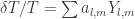
 are known as the multipole moments of the temperature distribution. Substituting this in the correlation function definition we obtain
 . We’re almost finished with our derivation! The final step is to convert from the correlation function to it’s momentum space representation, known as the power spectrum. With a little work, you can show that the power at multipole number
  is given by


 strings at next-to-leading order. Mercifully, the ambitwistor string is far more well-behaved. The resulting amplitudes are rather
  -loop level. The resulting concept of off-shell scattering equations piqued my interest – I’ve set myself a challenge to use them in the next 12 months!
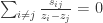
 are just two particle invariants – encoding things you can measure about the speed and angle of particle scattering. And the
  are just some bonus variables. You’d never dream of introducing them unless somebody told you to! But yet they’re exactly what’s required for a truly elegant description.
 form, ripe for
  dimensions. For technical reasons this is equivalent to working in the theory with an infinite number of color charges, not just the usual


 the square of the

 and
and  .
. . This is just an excitation of the string which generalizes electromagnetic potential.
 symmetry to
  where
where  is the dimension of your torus. Importantly for this to work, we must choose a
  metric get mixed up. This can have dramatic consequences for the underlying geometry! In particular our new metric may not patch together by diffeomorphisms on our spacetime. Similarly our new Kalb-Ramond field
  group does not embed within the group of generalized diffeomorphisms of our spacetime!
 . If we want a Killing vector
  to generate an overall symmetry then we’d better have

