It’s time to prove the central result of elementary algebraic geometry. Mostly it’s referred to as Hilbert’s Nullstellensatz. This German term translates precisely to the title of this post. Indeed ‘Null’ means ‘zero’, ‘stellen’ means to exist and ‘Satz’ means theorem. But referring to it merely as an existence theorem for zeroes is inadequate. Its real power is in setting up a correspondence between algebra and geometry.
Are you sitting comfortably? Grab a glass of water (or wine if you prefer). Settle back and have a peruse of these theorems. This is your first glance into the heart of a magical subject.
(In many texts these theorems are all referred to as the Nullstellensatz. I think this is both pointless and confusing, so have renamed them! If you have any comments or suggestions about these names please let me know).
Theorem 4.1 (Hilbert’s Nullstellensatz) Let ![J\subsetneq k[\mathbb{A}^n]](https://s0.wp.com/latex.php?latex=J%5Csubsetneq+k%5B%5Cmathbb%7BA%7D%5En%5D&bg=ffffff&fg=2b2b2b&s=0&c=20201002) be a proper ideal of the polynomial ring. Then
be a proper ideal of the polynomial ring. Then  . In other words, for every nontrivial ideal there exists a point which simulataneously zeroes all of its elements.
Theorem 4.2 (Maximal Ideal Theorem) Every maximal ideal ![\mathfrak{m}\subset k[\mathbb{A}^n]](https://s0.wp.com/latex.php?latex=%5Cmathfrak%7Bm%7D%5Csubset+k%5B%5Cmathbb%7BA%7D%5En%5D&bg=ffffff&fg=2b2b2b&s=0&c=20201002) is of the form
is of the form  for some
  . In other words every maximal ideal is the ideal of some single point in affine space.
Theorem 4.3 (Correspondence Theorem) For every ideal ![J\subset k[\mathbb{A}^n]](https://s0.wp.com/latex.php?latex=J%5Csubset+k%5B%5Cmathbb%7BA%7D%5En%5D&bg=ffffff&fg=2b2b2b&s=0&c=20201002) we have
we have  .
.
We’ll prove all of these shortly. Before that let’s have a look at some particular consequences. First note that 4.1 is manifestly false if  is not algebraically closed. Consider for example
  and
and  . Then certainly
  . Right then. From here on in we really must stick just to algebraically closed fields.
Despite having the famous name, 4.1 not really immediately useful. In fact we’ll see its main role is as a convenient stopping point in the proof of 4.3 from 4.2. The maximal ideal theorem is much more important. It precisely provides the converse to Theorem 3.10. But it is the correspondence theorem that is of greatest merit. As an immediate corollary of 4.3, 3.8 and 3.10 (recalling that prime and maximal ideals are radical) we have
Corollary 4.4 The maps  as defined in 1.2 and 2.4 give rise to the following bijections
![\{\textrm{affine varieties in }\mathbb{A}^n\} \leftrightarrow \{\textrm{radical ideals in } k[\mathbb{A}^n]\}](https://s0.wp.com/latex.php?latex=%5C%7B%5Ctextrm%7Baffine+varieties+in+%7D%5Cmathbb%7BA%7D%5En%5C%7D+%5Cleftrightarrow+%5C%7B%5Ctextrm%7Bradical+ideals+in+%7D+k%5B%5Cmathbb%7BA%7D%5En%5D%5C%7D&bg=ffffff&fg=2b2b2b&s=0&c=20201002)
![\{\textrm{irreducible varieties in }\mathbb{A}^n\} \leftrightarrow \{\textrm{prime ideals in } k[\mathbb{A}^n]\}](https://s0.wp.com/latex.php?latex=%5C%7B%5Ctextrm%7Birreducible+varieties+in+%7D%5Cmathbb%7BA%7D%5En%5C%7D+%5Cleftrightarrow+%5C%7B%5Ctextrm%7Bprime+ideals+in+%7D+k%5B%5Cmathbb%7BA%7D%5En%5D%5C%7D&bg=ffffff&fg=2b2b2b&s=0&c=20201002)
![\{\textrm{points in }\mathbb{A}^n\} \leftrightarrow \{\textrm{maximal ideals in } k[\mathbb{A}^n]\}](https://s0.wp.com/latex.php?latex=%5C%7B%5Ctextrm%7Bpoints+in+%7D%5Cmathbb%7BA%7D%5En%5C%7D+%5Cleftrightarrow+%5C%7B%5Ctextrm%7Bmaximal+ideals+in+%7D+k%5B%5Cmathbb%7BA%7D%5En%5D%5C%7D&bg=ffffff&fg=2b2b2b&s=0&c=20201002)
Proof We’ll prove the first bijection explicitly, for it is so rarely done in the literature. The second and third bijections follow from the argument for the first and 3.8, 3.10. Let  be a radical ideal in
 ![k[\mathbb{A}^n]](https://s0.wp.com/latex.php?latex=k%5B%5Cmathbb%7BA%7D%5En%5D&bg=ffffff&fg=2b2b2b&s=0&c=20201002) . Then
. Then  certainly an affine variety so
  well defined. Moreover is injective. For suppose
  radical with
  . Then
  and thus by 4.3
  . It remains to prove that surjective. Take
  an affine variety. Then
  an ideal with
  by Lemma 2.5. But
  not necessarily radical. Let
  a radical ideal. Then by 4.3
  . So
. So  by 2.5. This completes the proof.
We’ll see in the next post that we need not restrict our attention to  . In fact using the coordinate ring we can gain a similar correspondence for the subvarieties of any given variety. This will lead to an advanced introduction to the language of schemes. With these promising results on the horizon, let’s get down to business. We’ll begin by recalling a definition and a theorem.
Definition 4.5 A finitely generated -algebra is a ring  s.t.
s.t. ![R \cong k[a_1,\dots,a_n]](https://s0.wp.com/latex.php?latex=R+%5Ccong+k%5Ba_1%2C%5Cdots%2Ca_n%5D&bg=ffffff&fg=2b2b2b&s=0&c=20201002) for some
for some  . A finite -algebra is a ring s.t.
  .
.
Observe how this definition might be confusing when compared to a finitely generated -module. But applying a broader notion of ‘finitely generated’ to both algebras and modules clears up the issue. You can check that the following definition is equivalent to those we’ve seen for algebras and modules. A finitely generated algebra is richer than a finitely generated module because an algebra has an extra operation – multiplication.
Definition 4.6 We say an algebra (module)  is finitely generated if there exists a finite set of generators
  s.t. is the smallest algebra (module) containing . We then say that is generated by .
Theorem 4.7 Let be a general field and a finitely generated -algebra. If is a field then is algebraic over .
Okay I cheated a bit saying ‘recall’ Theorem 4.7. You probably haven’t seen it anywhere before. And you might think that it’s a teensy bit abstract! Nevertheless we shall see that it has immediate practical consequences. If you are itching for a proof, don’t worry. We’ll in fact present two. The first will be due to Zariski, and the second an idea of Noether. But before we come to those we must deduce 4.1 – 4.3 from 4.7.
Proof of 4.2 Let ![m \subset k[\mathbb{A}^n]](https://s0.wp.com/latex.php?latex=m+%5Csubset+k%5B%5Cmathbb%7BA%7D%5En%5D&bg=ffffff&fg=2b2b2b&s=0&c=20201002) be a maximal ideal. Then
be a maximal ideal. Then ![F = k[\mathbb{A}^n]/m](https://s0.wp.com/latex.php?latex=F+%3D+k%5B%5Cmathbb%7BA%7D%5En%5D%2Fm&bg=ffffff&fg=2b2b2b&s=0&c=20201002) a field. Define the natural homomorphism
a field. Define the natural homomorphism ![\pi: k[\mathbb{A}^n] \ni x \mapsto x+m \in F](https://s0.wp.com/latex.php?latex=%5Cpi%3A+k%5B%5Cmathbb%7BA%7D%5En%5D+%5Cni+x+%5Cmapsto+x%2Bm+%5Cin+F&bg=ffffff&fg=2b2b2b&s=0&c=20201002) . Note is a finitely generated -algebra, generated by the
. Note is a finitely generated -algebra, generated by the  certainly. Thus by 4.7
  is an algebraic extension. But was algebraically closed. Hence is isomorphic to via
 ![\phi : k \rightarrowtail k[\mathbb{A}^n] \xrightarrow{\pi} F](https://s0.wp.com/latex.php?latex=%5Cphi+%3A+k+%5Crightarrowtail+k%5B%5Cmathbb%7BA%7D%5En%5D+%5Cxrightarrow%7B%5Cpi%7D+F&bg=ffffff&fg=2b2b2b&s=0&c=20201002) .
.
Let  . Then
  so
so  . Hence
  . But
. But  is itself maximal by 3.10. Hence
  as required.
That was really quite easy! We just worked through the definitions, making good use of our stipulation that is algebraically closed. We’ll soon see that all the algebraic content is squeezed into the proof of 4.7
Proof of 4.1 Let be a proper ideal in the polynomial ring. Since Noetherian  some maximal ideal. From 4.2 we know that
  some point
  . Recall from 2.5 that
  so
so  .
.
The following proof is lengthier but still not difficult. Our argument uses a method known as the Rabinowitsch trick.
Proof of 4.3 Let ![J\triangleleft k[\mathbb{A}^n]](https://s0.wp.com/latex.php?latex=J%5Ctriangleleft+k%5B%5Cmathbb%7BA%7D%5En%5D&bg=ffffff&fg=2b2b2b&s=0&c=20201002) and
and  . We want to prove that
  s.t.
s.t.  . We start by introducing a new variable
  . Define an ideal
  by
by ![J_f = (J, ft - 1) \subset k[x_1,\dots,x_n,t]](https://s0.wp.com/latex.php?latex=J_f+%3D+%28J%2C+ft+-+1%29+%5Csubset+k%5Bx_1%2C%5Cdots%2Cx_n%2Ct%5D&bg=ffffff&fg=2b2b2b&s=0&c=20201002) . By definition
. By definition  . Note that
  so
so  .
.
Now by 4.1 we must have that  improper. In other words
 ![J_f = k[x_1,\dots, x_n, t]](https://s0.wp.com/latex.php?latex=J_f+%3D+k%5Bx_1%2C%5Cdots%2C+x_n%2C+t%5D&bg=ffffff&fg=2b2b2b&s=0&c=20201002) . In particular
. In particular  . Since
 ![k[x_1,\dots, x_n, t]](https://s0.wp.com/latex.php?latex=k%5Bx_1%2C%5Cdots%2C+x_n%2C+t%5D&bg=ffffff&fg=2b2b2b&s=0&c=20201002) is Noetherian we know that finitely generated by some
is Noetherian we know that finitely generated by some  say. Thus we can write
  where
where ![g_i\in k[x_1,\dots , x_n, t]](https://s0.wp.com/latex.php?latex=g_i%5Cin+k%5Bx_1%2C%5Cdots+%2C+x_n%2C+t%5D&bg=ffffff&fg=2b2b2b&s=0&c=20201002) (*).
(*).
Let  be such that
  is the highest power of appearing among the
  for
for  . Now multiplying (*) above by
  yields
  where we define
  . This equation is valid in
 ![k[x_1,\dots,x_n, t]](https://s0.wp.com/latex.php?latex=k%5Bx_1%2C%5Cdots%2Cx_n%2C+t%5D&bg=ffffff&fg=2b2b2b&s=0&c=20201002) . Consider its reduction in the ring
. Consider its reduction in the ring ![k[x_1,\dots,x_n,t]/(ft - 1)](https://s0.wp.com/latex.php?latex=k%5Bx_1%2C%5Cdots%2Cx_n%2Ct%5D%2F%28ft+-+1%29&bg=ffffff&fg=2b2b2b&s=0&c=20201002) . We have the congruence
. We have the congruence  where
where  .
.
Now consider the map ![\phi:k[x_1,\dots, x_n]\rightarrowtail k[x_n,\dots, x_n,t]\xrightarrow{\pi} k[x_n,\dots, x_n,t]/(ft-1)](https://s0.wp.com/latex.php?latex=%5Cphi%3Ak%5Bx_1%2C%5Cdots%2C+x_n%5D%5Crightarrowtail+k%5Bx_n%2C%5Cdots%2C+x_n%2Ct%5D%5Cxrightarrow%7B%5Cpi%7D+k%5Bx_n%2C%5Cdots%2C+x_n%2Ct%5D%2F%28ft-1%29&bg=ffffff&fg=2b2b2b&s=0&c=20201002) . Certainly nothing in the image of the injection can possibly be in the ideal
. Certainly nothing in the image of the injection can possibly be in the ideal  , not having any dependence. Hence
  must be injective. But then we see that
  holds in the ring . Recalling that the
  generate gives the result.
We shall devote the rest of this post to establishing 4.7. To do so we’ll need a number of lemmas. You might be unable to see the wood for the trees! If so, you can safely skim over much of this. The important exception is Noether normalisation, which we’ll come to later. I’ll link the ideas of our lemmas to geometrical concepts at our next meeting.
Definition 4.8 Let  be rings with
  . Let
. Let  . We say that
  is integral over
  if is the root of some monic polynomial with roots in . That is to say
  s.t.
s.t.  . If every
  is integral over we say that is integral over or is an integral extension of .
Let’s note some obvious facts. Firstly we can immediately talk about being integral over when are algebras with a subalgebra of . Remember an algebra is still a ring! It’s rather pedantic to stress this now, but hopefully it’ll prevent confusion if I mix my termin0logy later. Secondly observe that when and are fields “integral over” means exactly the same as “algebraic over”.
We’ll begin by proving some results that will be of use in both our approaches. We’ll see that there’s a subtle interplay between finite -algebras, integral extensions and fields.
Lemma 4.9 Let be a field and  a subring. Suppose is an integral extension of . Then is itself a field.
Proof Let  . Then certainly
  so
so  since a field. Now
  integral over so satisfies an equation
  with
with . But now multiplying through by
  yields
  .
.
Note that this isn’t obvious a priori. The property that an extension is integral contains sufficient information to percolate the property of inverses down to the base ring.
Lemma 4.10 If is a finite algebra then is integral over .
Proof Write  . Let
. Let  . We want to prove that
  satisfies some equation
  . We’ll do so by appealing to our knowledge about determinants. For each
  we may clearly write
  for some
  .
.
Writing  and defining the matrix
  we can express our equation as
  . We recognise this as an eigenvalue problem. In particular satisfies the characteristic polynomial of
  , a polynomial of degree
  with coefficients in . But this is precisely what we wanted to show.
Corollary 4.11 Let be a field and  a subring. If is a finite -algebra then is itself a field.
Proof Immediate from 4.9 and 4.10.
We now focus our attention on Zariski’s proof of the Nullstellensatz. I take as a source Daniel Grayson’s excellent exposition.
Lemma 4.12 Let be a ring an a -algebra generated by  . Suppose further that a field. Then
  s.t.
s.t. ![S = R[s^{-1}]](https://s0.wp.com/latex.php?latex=S+%3D+R%5Bs%5E%7B-1%7D%5D&bg=ffffff&fg=2b2b2b&s=0&c=20201002) a field. Moreover is algebraic over
a field. Moreover is algebraic over  .
.
Proof Let  be the fraction field of . Now recall that is algebraic over iff
 ![R'[x] \supset R'(x)](https://s0.wp.com/latex.php?latex=R%27%5Bx%5D+%5Csupset+R%27%28x%29&bg=ffffff&fg=2b2b2b&s=0&c=20201002) . Thus is algebraic over iff
. Thus is algebraic over iff ![R'[x]](https://s0.wp.com/latex.php?latex=R%27%5Bx%5D&bg=ffffff&fg=2b2b2b&s=0&c=20201002) is a field. So certainly our is algebraic over for we are given that a field. Let
is a field. So certainly our is algebraic over for we are given that a field. Let  be the minimal polynomial of .
Now define  to be the common denominator of the , so that
 ![f_0,\dots, f_{n-1} \in R[s^{-1}] = S](https://s0.wp.com/latex.php?latex=f_0%2C%5Cdots%2C+f_%7Bn-1%7D+%5Cin+R%5Bs%5E%7B-1%7D%5D+%3D+S&bg=ffffff&fg=2b2b2b&s=0&c=20201002) . Now is integral over so
. Now is integral over so  an integral extension. But then by 4.9 a field, and algebraic over it.
Observe that this result is extremely close to 4.7. Indeed if we take to be a field we have  in 4.12. Then lemma then says that
 ![R[x]](https://s0.wp.com/latex.php?latex=R%5Bx%5D&bg=ffffff&fg=2b2b2b&s=0&c=20201002) is algebraic as a field extension of . Morally this proof mostly just used definitions. The only nontrivial fact was the relationship between
is algebraic as a field extension of . Morally this proof mostly just used definitions. The only nontrivial fact was the relationship between  and . Even this is not hard to show rigorously from first principles, and I leave it as an exercise for the reader.
We’ll now attempt to generalise 4.12 to ![R[x_1,\dots,x_n]](https://s0.wp.com/latex.php?latex=R%5Bx_1%2C%5Cdots%2Cx_n%5D&bg=ffffff&fg=2b2b2b&s=0&c=20201002) . The argument is essentially inductive, though quite laborious. 4.7 will be immediate once we have succeeded.
. The argument is essentially inductive, though quite laborious. 4.7 will be immediate once we have succeeded.
Lemma 4.13 Let ![R = F[x]](https://s0.wp.com/latex.php?latex=R+%3D+F%5Bx%5D&bg=ffffff&fg=2b2b2b&s=0&c=20201002) be a polynomial ring over a field . Let
be a polynomial ring over a field . Let  . Then
 ![R[u^{-1}]](https://s0.wp.com/latex.php?latex=R%5Bu%5E%7B-1%7D%5D&bg=ffffff&fg=2b2b2b&s=0&c=20201002) is not a field.
is not a field.
Proof By Euclid, has infinitely many prime elements. Let  be a prime not dividing
  . Suppose
 ![\exists q \in R[u^{-1}]](https://s0.wp.com/latex.php?latex=%5Cexists+q+%5Cin+R%5Bu%5E%7B-1%7D%5D&bg=ffffff&fg=2b2b2b&s=0&c=20201002) s.t.
s.t.  . Then
  where
where  a polynomial of degree with coefficients in . Hence in particular
  holds in for
  . Thus
  but prime so
  . This is a contradiction.
Corollary 4.14 Let  be a field,
  a subfield, and
  . Let . Suppose
  s.t.
s.t. ![R[u^{-1}] = K](https://s0.wp.com/latex.php?latex=R%5Bu%5E%7B-1%7D%5D+%3D+K&bg=ffffff&fg=2b2b2b&s=0&c=20201002) . Then is algebraic over . Moreover
. Then is algebraic over . Moreover  .
.
Proof Suppose were transcendental over . Then ![R=F[x]](https://s0.wp.com/latex.php?latex=R%3DF%5Bx%5D&bg=ffffff&fg=2b2b2b&s=0&c=20201002) would be a polynomial ring, so by 4.12 couldn’t be a field. Hence is algebraic over so is a field. Hence
would be a polynomial ring, so by 4.12 couldn’t be a field. Hence is algebraic over so is a field. Hence ![R=R[u{-1}]=K](https://s0.wp.com/latex.php?latex=R%3DR%5Bu%7B-1%7D%5D%3DK&bg=ffffff&fg=2b2b2b&s=0&c=20201002) .
.
The following fairly abstract theorem is the key to unlocking the Nullstellensatz. It’s essentially a slight extension of 4.14, applying 4.12 in the process. I’d recommend skipping the proof first time, focussing instead on how it’s useful for the induction of 4.16.
Theorem 4.15 Take a field,  a subring, . Let . Suppose s.t. . Then
 ![\exists 0\neq s \in F s.t. F[s^{-1}]](https://s0.wp.com/latex.php?latex=%5Cexists+0%5Cneq+s+%5Cin+F+s.t.+F%5Bs%5E%7B-1%7D%5D&bg=ffffff&fg=2b2b2b&s=0&c=20201002) is a field. Moreover
is a field. Moreover ![F[s^{-1}][x] = K](https://s0.wp.com/latex.php?latex=F%5Bs%5E%7B-1%7D%5D%5Bx%5D+%3D+K&bg=ffffff&fg=2b2b2b&s=0&c=20201002) and is algebraic over
and is algebraic over ![F[s^{-1}]](https://s0.wp.com/latex.php?latex=F%5Bs%5E%7B-1%7D%5D&bg=ffffff&fg=2b2b2b&s=0&c=20201002) .
.
Proof Let  . Now by 4.14 we can immediately say that
 ![L[x]=K](https://s0.wp.com/latex.php?latex=L%5Bx%5D%3DK&bg=ffffff&fg=2b2b2b&s=0&c=20201002) , with algebraic over
, with algebraic over  . Now we seek our element
  with the desired properties. Looking back at 4.12, we might expect it to be useful. But to use 4.12 for our purposes we’ll need to apply it to some
 ![F' = F[t^{-1}]](https://s0.wp.com/latex.php?latex=F%27+%3D+F%5Bt%5E%7B-1%7D%5D&bg=ffffff&fg=2b2b2b&s=0&c=20201002) with
with ![F'[x] = K](https://s0.wp.com/latex.php?latex=F%27%5Bx%5D+%3D+K&bg=ffffff&fg=2b2b2b&s=0&c=20201002) , where
, where  .
.
Suppose we’ve found such a . Then 4.12 gives us  s.t.
s.t. ![F'[s'^{-1}]](https://s0.wp.com/latex.php?latex=F%27%5Bs%27%5E%7B-1%7D%5D&bg=ffffff&fg=2b2b2b&s=0&c=20201002) a field with algebraic over it. But now
a field with algebraic over it. But now  some
some  . Now
. Now ![F'[s'^{-1}]=F[t^{-1}][s'^{-1}]=F[(qt)^{-1}]](https://s0.wp.com/latex.php?latex=F%27%5Bs%27%5E%7B-1%7D%5D%3DF%5Bt%5E%7B-1%7D%5D%5Bs%27%5E%7B-1%7D%5D%3DF%5B%28qt%29%5E%7B-1%7D%5D&bg=ffffff&fg=2b2b2b&s=0&c=20201002) , so setting
, so setting  completes the proof. (You might want to think about that last equality for a second. It’s perhaps not immediately obvious).
So all we need to do is find . We do this using our first observation in the proof. Observe that ![u^{-1}\in K=L[x]](https://s0.wp.com/latex.php?latex=u%5E%7B-1%7D%5Cin+K%3DL%5Bx%5D&bg=ffffff&fg=2b2b2b&s=0&c=20201002) so we can write
so we can write  ,
,  . Now let be a common denominator for all the
  . Then
 ![u^{-1} \in F'=F[t^{-1}]](https://s0.wp.com/latex.php?latex=u%5E%7B-1%7D+%5Cin+F%27%3DF%5Bt%5E%7B-1%7D%5D&bg=ffffff&fg=2b2b2b&s=0&c=20201002) so
so ![F'[x]=K](https://s0.wp.com/latex.php?latex=F%27%5Bx%5D%3DK&bg=ffffff&fg=2b2b2b&s=0&c=20201002) as required.
as required.
Corollary 4.16 Let a ring, a field, finitely generated as a -algebra by  . Then
  s.t.
s.t. ![k[s^{-1}]](https://s0.wp.com/latex.php?latex=k%5Bs%5E%7B-1%7D%5D&bg=ffffff&fg=2b2b2b&s=0&c=20201002) a field, with a finite algebraic extension of . Trivially if a field, then is algebraic over , establishing 4.7.
a field, with a finite algebraic extension of . Trivially if a field, then is algebraic over , establishing 4.7.
Proof Apply Lemma 4.15 with ![F=k[x_1,\dots,x_{n-1}]](https://s0.wp.com/latex.php?latex=F%3Dk%5Bx_1%2C%5Cdots%2Cx_%7Bn-1%7D%5D&bg=ffffff&fg=2b2b2b&s=0&c=20201002) ,
,  ,
,  to get
  s.t.
s.t. ![A' = k[x_1,\dots,x_{n-1}][s'^{-1}]](https://s0.wp.com/latex.php?latex=A%27+%3D+k%5Bx_1%2C%5Cdots%2Cx_%7Bn-1%7D%5D%5Bs%27%5E%7B-1%7D%5D&bg=ffffff&fg=2b2b2b&s=0&c=20201002) is a field with
is a field with  algebraic over it. But now apply 4.15 again with
 ![F=k[x_1,\dots,x_{n-2}]](https://s0.wp.com/latex.php?latex=F%3Dk%5Bx_1%2C%5Cdots%2Cx_%7Bn-2%7D%5D&bg=ffffff&fg=2b2b2b&s=0&c=20201002) ,
,  to deduce that
 ![A''=k[x_1,\dots, x_{n-2}][s''^{-1}]](https://s0.wp.com/latex.php?latex=A%27%27%3Dk%5Bx_1%2C%5Cdots%2C+x_%7Bn-2%7D%5D%5Bs%27%27%5E%7B-1%7D%5D&bg=ffffff&fg=2b2b2b&s=0&c=20201002) is a field, with
is a field, with  algebraic over
  , for some
  . Applying the lemma a further
  times gives the result.
This proof of the Nullstellensatz is pleasingly direct and algebraic. However it has taken us a long way away from the geometric content of the subject. Moreover 4.13-4.15 are pretty arcane in the current setting. (I’m not sure whether they become more meaningful with a better knowledge of the subject. Do comment if you happen to know)!
Our second proof sticks closer to the geometric roots. We’ll introduce an important idea called Noether Normalisation along the way. For that you’ll have to come back next time!


![\displaystyle S[X,\gamma]= \int d^{p+1}\xi \sqrt{|\gamma|}\left(\gamma^{ij}g_{ij}+(1-p)\right)](https://s0.wp.com/latex.php?latex=%5Cdisplaystyle+S%5BX%2C%5Cgamma%5D%3D+%5Cint+d%5E%7Bp%2B1%7D%5Cxi+%5Csqrt%7B%7C%5Cgamma%7C%7D%5Cleft%28%5Cgamma%5E%7Bij%7Dg_%7Bij%7D%2B%281-p%29%5Cright%29&bg=ffffff&fg=2b2b2b&s=0&c=20201002)


 during renormalization. The
 the renormalization scale. At a fixed point
  of the renormalization group flow, it can be shown that
  exactly encodes the difference between the classical dimension of
  -loop calculations. Despite all this hoodoo, I have failed to provide a single example of a successful application. Now it’s time for that to change. I’m about to show you just how useful generalized unitarity can be, borrowing examples from
  Yang-Mills (YM).
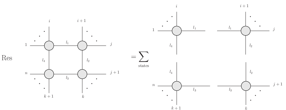
 are taken on-shell. On the right hand side, I take a product of tree level diagrams with external lines as shown, and sum over the possible particle content of the
  dimensions could be expressed as linear combinations of scalar loop diagrams with
  sides. Later Bern, Dixon and Kosower
 are integrals corresponding to particular scalar theory diagrams,
  indicate distribution of momenta on external legs,
  is a rational function and
  a regulator.
 ,
,  and
and  are referred to as box, triangle and bubble integrals respectively. This is an obvious homage to their structure as Feynman diagrams. For example a triangle diagram looks like
 ,
,  ,
,  label the sums of external momenta at each of the vertices. The Feynman rules give (in dimensional regularization)
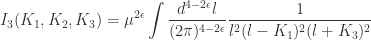
 above an integral basis expansion. It’s useful because the integrands of box, triangle and bubble diagrams have different pole structures. Thus we can reconstruct their coefficients by taking generalized unitarity cuts. Of course, the rational term cannot be determined this way. Theoretically we have reduced our problem to a simpler case, but not completely solved it.
 . Such terms will be familiar if you’ve studied anomalies.
 -point
  ,
,  and
and  .
.
 is the tree level
  ve helicity. Leaving the momentum conservation delta function implicit we quote the standard result
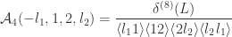
 is a supermomentum conservation delta function. We get a similar result for the other tree level amplitude, involving a delta function
  . Now by definition of the superamplitude, the sum over states can be effected as an integral over the Grassman variables
  and
and  . Under the integral signs we may write
 is the overall supermomentum conservation delta function, which one can always factor out of a superamplitude in a supersymmetric theory. The remaining delta function gives a nonzero contribution in the integral. To evaluate this recall that the Grassman delta function for a process with
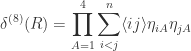


 and
and  . But which basis integrands contribute to the residue from our unitarity cut?
 appears as factors of
  . These may be immediately matched with uncut loop propagators in the basis diagrams. Simple counting then establishes which basis diagram we want. As an example
 . To accomplish this, we must express the residue
  in more familiar momentum space variables. Our tools are the trusty identities
![\displaystyle \langle ij \rangle [ij] =(p_i + p_j)^2](https://s0.wp.com/latex.php?latex=%5Cdisplaystyle+%5Clangle+ij+%5Crangle+%5Bij%5D+%3D%28p_i+%2B+p_j%29%5E2&bg=ffffff&fg=2b2b2b&s=0&c=20201002)
![\displaystyle \sum_i \langle ri \rangle [ik] = 0](https://s0.wp.com/latex.php?latex=%5Cdisplaystyle+%5Csum_i+%5Clangle+ri+%5Crangle+%5Bik%5D+%3D+0&bg=ffffff&fg=2b2b2b&s=0&c=20201002)
 relation.
 . This leaves us with
![[l_2 2]](https://s0.wp.com/latex.php?latex=%5Bl_2+2%5D&bg=ffffff&fg=2b2b2b&s=0&c=20201002) . A quick round of momentum conservation leaves us with
. A quick round of momentum conservation leaves us with![\displaystyle \textrm{Res}_s = \mathcal{A}_4^{\textrm{tree}} \frac{\langle 23 \rangle \langle 41 \rangle [12] \langle l_1 l_2 \rangle}{(l_2 + p_2)^2\langle l_2 4 \rangle \langle 3 l_1 \rangle}](https://s0.wp.com/latex.php?latex=%5Cdisplaystyle+%5Ctextrm%7BRes%7D_s+%3D+%5Cmathcal%7BA%7D_4%5E%7B%5Ctextrm%7Btree%7D%7D+%5Cfrac%7B%5Clangle+23+%5Crangle+%5Clangle+41+%5Crangle+%5B12%5D+%5Clangle+l_1+l_2+%5Crangle%7D%7B%28l_2+%2B+p_2%29%5E2%5Clangle+l_2+4+%5Crangle+%5Clangle+3+l_1+%5Crangle%7D&bg=ffffff&fg=2b2b2b&s=0&c=20201002)
![[3l_1]](https://s0.wp.com/latex.php?latex=%5B3l_1%5D&bg=ffffff&fg=2b2b2b&s=0&c=20201002) . Again momentum conservation leaves us with
. Again momentum conservation leaves us with![\displaystyle \textrm{Res}_s = \mathcal{A}_4^{\textrm{tree}} \frac{\langle 23 \rangle \langle 41 \rangle [12] [34]}{(l_2 + p_2)^2 (l_1+p_3)^2}](https://s0.wp.com/latex.php?latex=%5Cdisplaystyle+%5Ctextrm%7BRes%7D_s+%3D+%5Cmathcal%7BA%7D_4%5E%7B%5Ctextrm%7Btree%7D%7D+%5Cfrac%7B%5Clangle+23+%5Crangle+%5Clangle+41+%5Crangle+%5B12%5D+%5B34%5D%7D%7B%28l_2+%2B+p_2%29%5E2+%28l_1%2Bp_3%29%5E2%7D&bg=ffffff&fg=2b2b2b&s=0&c=20201002)
![\displaystyle \textrm{Res}_s = -\mathcal{A}_4^{\textrm{tree}} \frac{\langle 12 \rangle [12] \langle 23 \rangle [23]}{(l_2 + p_2)^2 (l_1+p_3)^2} = -\mathcal{A}_4^{\textrm{tree}} \frac{st}{(l_2 + p_2)^2 (l_1+p_3)^2}](https://s0.wp.com/latex.php?latex=%5Cdisplaystyle+%5Ctextrm%7BRes%7D_s+%3D+-%5Cmathcal%7BA%7D_4%5E%7B%5Ctextrm%7Btree%7D%7D+%5Cfrac%7B%5Clangle+12+%5Crangle+%5B12%5D+%5Clangle+23+%5Crangle+%5B23%5D%7D%7B%28l_2+%2B+p_2%29%5E2+%28l_1%2Bp_3%29%5E2%7D+%3D+-%5Cmathcal%7BA%7D_4%5E%7B%5Ctextrm%7Btree%7D%7D+%5Cfrac%7Bst%7D%7B%28l_2+%2B+p_2%29%5E2+%28l_1%2Bp_3%29%5E2%7D&bg=ffffff&fg=2b2b2b&s=0&c=20201002)


 throughout this post. Recall that Feynman rules usually assign a factor of
  . This precisely corrects the sign error than pedants (or experimentalists) would find irritating!
 negative helicity external gluons and
  positive helicity ones. The four-mass condition means that each corner of the box has more than two external legs, so that the outgoing momentum is a massive
  negative helicity gluons to go round.
 legs must have at least
  negative helicity gluons to be non-vanishing. This is not possible with our setup, since
  . We conclude that the NMHV gluon four-mass box coefficients vanish.
 .
. prescription yields an imaginary contribution.


 -matrix defined by
 yields for the

 term? Thinking back to the heady days of elementary quantum mechanics, perhaps you’re inspired to try inserting a completeness relation in the middle. That way you obtain a product of amplitudes, which are things we know how to compute. The final result looks like

 viz.
viz.
 is the
  incoming and


 ,
,  and have left implicit a sum over the possible intermediate states. This result is certainly curious, but it’s hard to see how it can be useful in its current form. In particular, the sum we left implicit involves an arbitrary number of states. We’d really like a simpler relation which involves a well-defined, finite number of Feynman diagrams.
![S = k[x_1,\dots,x_n]](https://s0.wp.com/latex.php?latex=S+%3D+k%5Bx_1%2C%5Cdots%2Cx_n%5D&bg=ffffff&fg=2b2b2b&s=0&c=20201002) and a group
and a group  acting on
  and note that it certainly forms a subalgebra of
  be an ideal in the image under than homomorphism
  an ideal in
  and
and  then
then  so
so  . Hence
  to a generator of
  is Noetherian if every submodule
  with coefficients in
  , and let
  then clearly the map
  defined by
  is surjective. Then the preimage of
  . (*)
. (*) . Consider the quotient map
  . Let
. Let  be the image of
  . Let
. Let  be elements of
  is a submodule of
  is finitely generated, by
  say.
say. generate
  the image of
  which is precisely a linear combination of the
  by construction. This completes the induction.
  and
and  . As in our notation above, we take
 ![S=k[x_1,\dots,x_n]](https://s0.wp.com/latex.php?latex=S%3Dk%5Bx_1%2C%5Cdots%2Cx_n%5D&bg=ffffff&fg=2b2b2b&s=0&c=20201002) .
. , which of course can naturally be seen as the group of invertible linear transformations of the vector space
  . This is in fact the definition of a representation of
  .
. or
or  we shall further suppose that our representation of
  act on
  from
from  . Thus we may view
  of homogeneous forms of degree
  , such that
  .
. as our indexing set for the
  , and such graded rings are often called
  we have a unique expression for
  with
with  . (I have yet to convince myself why this terminates generally, any thoughts? I’ve also asked
  .
. with
with  containing all the forms (homogeneous polynomials) of degree
  . Let
. Let  be a homogeneous element. Then we may write
  with
with  .
. with
with  . Take
  of degree
  maps
maps  of
of  . Note that we have implicitly used that
  exists. In the case that
  .
. be the ideal of
  . By the Basis Theorem
  an ideal of
  which we may wlog assume lie in
  a general homogeneous polynomial. Suppose we have shown
  . Let
. Let  a sum of homogeneous components. But
  also, and we are done.
 which we’ll do by induction on the degree of
  then
then  . Suppose
  so
so  by Lemma A.10. But again we may use the map
  for
for  . But
. But  0f lower degree than
  and hence
  a Noetherian graded ring iff
  Noetherian and
  . These crop up all the time in maths and there’s a lot of them. Go onto
  that we say last time is a good example of a hypersurface. Finally we say a hyperplane is the zero of a single polynomial of degree
  that aren’t algebraic varieties. A simple observation allows us to come up with a huge class of such subsets. Recall that polynomials are continuous functions from
  , and therefore their zero sets must be closed in the Euclidean topology. Hence in particular, no open ball in
  is not an affine variety. Secondly the closed square
  is an example of a closed set which is not an affine variety. This is because it clearly contains interior points, while no affine variety in
  can contain such points. I’m not entirely sure at present why this is, so I’ve
  s.t.
s.t.  for all
  .
.![N[x_1]](https://s0.wp.com/latex.php?latex=N%5Bx_1%5D&bg=ffffff&fg=2b2b2b&s=0&c=20201002) is Noetherian also, and by induction so is
is Noetherian also, and by induction so is ![N[x_1,\dots,x_n]](https://s0.wp.com/latex.php?latex=N%5Bx_1%2C%5Cdots%2Cx_n%5D&bg=ffffff&fg=2b2b2b&s=0&c=20201002) for any positive integer
for any positive integer ![I\subset k[\mathbb{A}^n]](https://s0.wp.com/latex.php?latex=I%5Csubset+k%5B%5Cmathbb%7BA%7D%5En%5D&bg=ffffff&fg=2b2b2b&s=0&c=20201002) as
as  for some finite
  , using the ascending chain condition. Why is this useful? For that we’ll need a lemma.
 be an affine variety, so
  some
some ![T\subset K[\mathbb{A}^n]](https://s0.wp.com/latex.php?latex=T%5Csubset+K%5B%5Cmathbb%7BA%7D%5En%5D&bg=ffffff&fg=2b2b2b&s=0&c=20201002) . Let
. Let  , the ideal generated by
  .
. so
so  . We now need to show the reverse inclusion. For any
  there exist polynomials
  in
in  in
in ![K[\mathbb{A}^n]](https://s0.wp.com/latex.php?latex=K%5B%5Cmathbb%7BA%7D%5En%5D&bg=ffffff&fg=2b2b2b&s=0&c=20201002) s.t.
s.t.  . Hence if
  then
then  so
so  .
.  . If you don’t get this straight away look back carefully at the theorem and the lemma. Can you see how to marry their conclusions to get this fact?
 we say the ideal of
 ![I(X):=\{f \in k[\mathbb{A}^n] : f(x)=0\forall x\in X\}](https://s0.wp.com/latex.php?latex=I%28X%29%3A%3D%5C%7Bf+%5Cin+k%5B%5Cmathbb%7BA%7D%5En%5D+%3A+f%28x%29%3D0%5Cforall+x%5Cin+X%5C%7D&bg=ffffff&fg=2b2b2b&s=0&c=20201002) .
. . Try to think of some other obvious examples before we move on.
![V: \{\textrm{ideals in }k[\mathbb{A}^n]\}\rightarrow \{\textrm{affine varieties in }\mathbb{A}^n\}](https://s0.wp.com/latex.php?latex=V%3A+%5C%7B%5Ctextrm%7Bideals+in+%7Dk%5B%5Cmathbb%7BA%7D%5En%5D%5C%7D%5Crightarrow+%5C%7B%5Ctextrm%7Baffine+varieties+in+%7D%5Cmathbb%7BA%7D%5En%5C%7D&bg=ffffff&fg=2b2b2b&s=0&c=20201002) and
and ![I:\{\textrm{subsets of }\mathbb{A}^n\}\rightarrow \{\textrm{ideals in }k[\mathbb{A}^n]\}](https://s0.wp.com/latex.php?latex=I%3A%5C%7B%5Ctextrm%7Bsubsets+of+%7D%5Cmathbb%7BA%7D%5En%5C%7D%5Crightarrow+%5C%7B%5Ctextrm%7Bideals+in+%7Dk%5B%5Cmathbb%7BA%7D%5En%5D%5C%7D&bg=ffffff&fg=2b2b2b&s=0&c=20201002) . Intuitively these maps are somehow ‘opposite’ to each other. We’d like to be able to formalise that mathematically. More specifically we want to find certain classes of affine varieties and ideals where
. Intuitively these maps are somehow ‘opposite’ to each other. We’d like to be able to formalise that mathematically. More specifically we want to find certain classes of affine varieties and ideals where  , but
, but  so
so  we see that
  so
so  so
so  ideals and
  subsets of


 with equality iff
  is an affine variety
 “. Let
  . Wlog assume
  . Then
  . So certainly
  , which is what we needed to prove. Now we show “
 “. Let
  . Then
  and
and  . So there exists
  s.t.
s.t.  . Hence
  . But
. But  s0
s0  .
. , and then it’s trivial.
 then
then  by definition, so
  .
. , some ideal
  . Then by (5)
  . Conversely, suppose
  . Then
  so an affine variety by definition.
  bijections will give us a dictionary between algebra and geometry. With minimal effort we can translate problems into an easier language. In particular, we’ll be allowed to use a generous dose of algebra to sweeten the geometric cocktail! You’ll have to wait until next time to see that in all its glory.
 we can make some comparisons with the usual Euclidean topology.
 ) in the Euclidean topology. In particular, no nonempty Zariski open set is bounded in the Euclidean topology. Hence we immediately see that the intersection of two nonempty Zariski open sets of
  ^n is never empty. This important observation tells us the the Zariski topology is not Hausdorff. We really are working with a very strange topological space!