Scattering Without Scale, Or The S-Matrix In N=4

My research focuses on an unrealistic theory called massless super Yang-Mills (SYM). This sounds pretty pointless, at least at first. But actually this model shares many features with more complete accounts of reality.  So it’s not all pie in the sky.

The reason I look at  SYM is because it contains lots of symmetry. This simplifies matters a lot. Studying SYM is like going to an adventure playground – you can still have great fun climbing and jumping, but it’s a lot safer than roaming out into a nearby forest.

Famously SYM has a conformal symmetry. Roughly speaking, this means that the theory looks the same at every length scale. (Whether conformal symmetry is equivalent to scale invariance is a hot topic, in fact)! Put another way, SYM has no real notion of length. I told you it was unrealistic.

This is a bit unfortunate for me, because I’d like to use SYM to think about particle scattering. To understand the problem, you need to know what I want to calculate. The official name for this quantity is the S-matrix.

The jargon is quite straightforward. “S” just stands for scattering. The “matrix” part tells you that this quantity encodes many possible scattering outcomes. To get an S-matrix, you have to assume you scatter particles from far away. That’s certainly the case in big particle accelerators – the LHC is huge compared to a proton!

But remember I said that SYM doesn’t have a length scale. So really you can’t get an S-matrix. And without an S-matrix, you can’t say anything about particle scattering. Things aren’t looking good.

Fortunately all is not lost. You can try to define an S-matrix using the usual techniques that worked in normal theories. All the calculations go through fine, unless there are any low energy particles around. Any of these so-called soft particles will cause your S-matrix to blow up to infinity!

But hey, we should expect our S-matrix to be badly behaved. After all, we’ve chosen a theory without a sense of scale! These irritating infinities go by the name of infrared divergences. Thankfully there’s a systematic way of eliminating them.

Remember that I said our SYM theory is massless. All the particles are like photons, constantly whizzing about that the speed of light. If you were a photon, life would be very dull. That’s because you’d move so fast through space you couldn’t move through time. This means that essentially our massless particles have no way of knowing about distances.

Viewed from this perspective it’s intuitive that this lack of mass yields the conformal symmetry. We can remove the troublesome divergences by destroying the conformal symmetry. We do this in a controlled way by giving some particles a small mass.

Technically our theory is now called Coulomb branch SYM. Who’s Coulomb, I hear you cry? He’s the bloke who developed electrostatics 250 years ago. And why’s he cropped up now? Because when we dispense with conformal symmetry, we’re left with some symmetries that match those of electromagnetism.

In Coulomb branch SYM it’s perfectly fine to define an S-matrix! You get sensible answers from all your calculations. Now imagine we try to recover our original theory by decreasing all masses to zero. Looking closely at the S-matrix, we see it split into two pieces – finite and infinite. Just ignore the infinite bit, and you’ve managed to extract useful scattering data for the original conformal theory!

You might think I’m a bit blasé in throwing away these divergences. But this is actually well-motivated physically. The reason is that such infinities cancel in any measurable quantity. You could say that they only appear in the first place because you’re doing the wrong sum!

This perspective has been formalized for the realistic theories as the KLN theorem. It may even be possible to get a rigorous version for our beloved massless SYM.

So next time somebody tells you that you can’t do scattering in a conformal theory, you can explain why they’re wrong! Okay, I grant you, that’s an unlikely pub conversation. But stranger things have happened.

And if you’re planning to grab a pint soon, make it a scientific one!

 

The Calculus of Particle Scattering

Quantum field theory allows us to calculate “amplitudes” for particle scattering processes. These are mathematical functions that encode the probability of particles scattering through various angles. Although the theory is quite complicated, miraculously the rules for calculating these amplitudes are pretty easy!

The key idea came from physicist Richard Feynman. To calculate a scattering amplitude, you draw a series of diagrams. The vertices and edges of the diagram come with particular factors relevant to the theory. In particular vertices usually carry coupling constants, external edges carry polarization vectors, and internal edges carry functions of momenta.

From the diagrams you can write down a mathematical expression for the scattering amplitude. All seems to be pretty simple. But what exactly are the diagrams you have to draw?

Well there are simple rules governing that too. Say you want to compute a scattering amplitude with incoming and outgoing particles. Then you draw four external lines, labelled with appropriate polarizations and momenta. Now you need to connect these lines up, so that they all become part of one diagram.

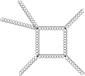
This involves adding internal lines, which connect to the external ones at vertices. The types and numbers of lines allowed to connect to a vertex is prescribed by the theory. For example in pure QCD the only particles are gluons. You are allowed to connect either three or four different lines to each vertex.

Here’s a few different diagrams you are allowed to draw – they each give different contributions to the overall scattering amplitude. Try to draw some more yourself if you’re feeling curious!

Now it’s immediately obvious that there are infinitely many possible diagrams you could draw. Sounds like this is a problem, because adding up infinitely many things is hard! Thankfully, we can ignore a lot of the diagrams.

So why’s that? Well it transpires that each loop in the diagram contributes an extra factor of Planck’s constant . This is a very small number, so the effect on the amplitude from diagrams with many loops is negligable. There are situations in which this analysis breaks down, but we won’t consider them here.

So we can get a good approximation to a scattering amplitude by evaluating diagrams with only a small number of loops. The simplest have -loops, and are known as tree level diagrams because they look like trees. Here’s a QCD example from earlier

Next up you have -loop diagrams. These are also known as quantum corrections because they give the QFT correction to scattering processes from quantum mechanics, which were traditionally evaluated using classical fields. Here’s a nice QCD -loop diagram from earlier

If you’ve been reading some of my recent posts, you’ll notice I’ve been talking about how to calculate tree level amplitudes. This is sensible because they give the most important contribution to the overall result. But the real reason for focussing on them is because the maths is quite easy.

Things get more complicated at -loop level because Feynman’s rules tell us to integrate over the momentum in the loop. This introduces another curve-ball for us to deal with. In particular our arguments for the simple tree level recursion relations now fail. It seems that all the nice tricks I’ve been learning are dead in the water when it comes to quantum corrections.

But thankfully, all is not lost! There’s a new set of tools that exploits the structure of -loop diagrams. Back in the 1950s Richard Cutkosky noticed that the -loop diagrams can be split into tree level ones under certain circumstances. This means we can build up information about loop processes from simpler tree results. The underlying principle which made this possible is called unitarity.

So what on earth is unitarity? To understand this we must return to the principles of quantum mechanics. In quantum theories we can’t say for definite what will happen. The best we can do is assign probabilities to different outcomes. Weird as this might sound, it’s how the universe seems to work at very small scales!

Probabilities measure the chances of different things happening. Obviously if you add up the chances of all possible outcomes you should get . Let’s take an example. Suppose you’re planning a night out, deciding whether to go out or stay in. Thinking back over the past few weeks you can estimate the probability of each outcome. Perhaps you stay in times out of and go out times out of ten. just as we’d expect for probability!

Now unitarity is just a mathsy way of saying that probabilities add up to . It probably sounds a bit stupid to make up a word for such a simple concept, but it’s a useful shorthand! It turns out that unitarity is exactly what we need to derive Cutkosky’s useful result. The method of splitting loop diagrams into tree level ones has become known as the unitarity method.

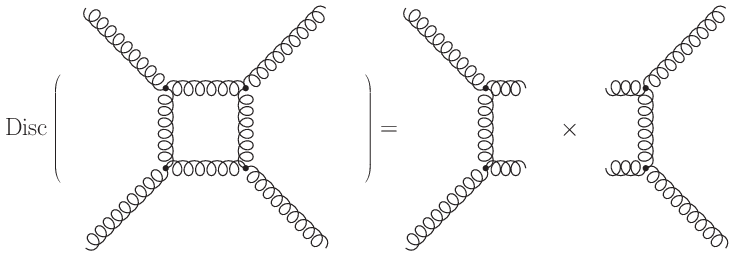
The nicest feature of this method is that it’s easy to picture in terms of Feynman diagrams. Let’s plunge straight in and see what that looks like.

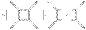
At first glance it’s not at all clear what this picture means. But it’s easy to explain step by step. Firstly observe that it’s an equation, just in image form. On the left hand side you see a loop diagram, accompanied by the word . This indicates a certain technical property of a loop diagram that it’s useful to calculate. On the right you see two tree diagrams multiplied together.

Mathematically these diagrams represent formulae for scattering amplitudes. So all this diagram says is that some property of -loop amplitudes is produced by multiplying together two tree level ones. This is extremely useful if you know about tree-level results but not about loops! Practically, people usually use this kind of equation to constrain the mathematical form of a -loop amplitude.

If you’re particularly sharp-eyed you might notice something about the diagrams on the left and right sides of the equation. The two diagrams on the right come from cutting through the loop on the left in two places. This cutting rule enables us to define the unitarity method for all loop diagrams. This gives us the full result that Cutkosky originally found. He’s perhaps the most aptly named scientist of all time!

We’re approaching the end of our whirlwind tour of particle scattering. We’ve seen how Feynman diagrams give simple rules but difficult maths. We’ve mentioned the tree level tricks that keep calculations easy. And now we’ve observed that unitarity comes to our rescue at loop-level. But most of these ideas are actually quite old. There’s just time for a brief glimpse of a hot contemporary technique.

In our pictorial representation of the unitarity method, we gained information by cutting the loop in two places. It’s natural to ask whether you could make further such cuts, giving more constraints on the form of the scattering amplitude. It turns out that the answer is yes, so long as you allow the momentum in the loop to be a complex number!

You’d be forgiven for thinking that this is all a bit unphysical, but in the previous post we saw that using the complex numbers is actually a very natural and powerful mathematical trick. The results we get in the end are still real, but the quickest route there is via the complex domain.

So why do the complex numbers afford us the extra freedom to cut more lines? Well, the act of cutting a line is mathematically equivalent to taking the corresponding momentum to be on-shell; that is to say . We live in a four-dimensional world, so has four components. That means we can solve a maximum of four equations simultaneously. So generically we should be allow to cut four lines!

However, the equations are quadratic. This means we are only guaranteed a solution if the momentum can be complex. So to use a four line cut, we must allow the loop momentum to be complex. With our simple line cuts there was enough freedom left to keep real.

The procedure of using several loop cuts is known as the generalized unitarity method. It’s been around since the late 90s, but is still actively used to determine scattering amplitudes. Much of our current knowledge about QCD loop corrections is down to the power of generalized unitarity!

That’s all for now folks. I’ll be covering the mathematical detail in a series of posts over the next few days.

My thanks to Binosi et al. for their excellent program JaxoDraw which eased the drawing of Feynman diagrams.

Complex Scattering For Beginners

Quantum field theory is a description of interacting particles. These are the fundamental constituents of our universe. They are real, in the sense that their properties are described by real numbers. For example, a typical particle has a momentum through spacetime described by a vector with four real components.

In my line of work we’re generally interested in finding out what happens when particles scatter. There are various rules that enable you to determine a numerical amplitude from diagrams of the process. These so-called “Feynman rules” combine the real quantities in different ways depending on the structure of the theory.

Trouble is, it can be quite tricky to do the exact calculations from these rules. It’s a bit like trying to put together a complicated piece of Ikea furniture with no idea what the end product is meant to look like! In a sense the task is possible, but you’d be hard pressed not to go wrong. Plus it would take you ages to finish the job.

What we really need is some extra pointers that tell us what we’re trying to build. Turns out that we can get that kind of information by performing a little trick. Instead of keeping all of our particle properties real, we bring in the complex numbers.

The complex numbers are like a souped up version of the real numbers. The extra ingredient is a new quantity which squares to . This might all sound rather contrived at the moment, but in fact mathematically the complex numbers are a lot nicer behaved. By bringing them into play you can extract more information about your original scattering process for free!

Let’s go back to our Ikea analogy. Suppose that you get a mate in to help with the job. Your task is still the same as ever, but now as you construct it you can share tips. This makes everything easier. Moreover you can pool your guesses about what piece of furniture you’re building. The end result is still the same (hopefully!) but the extra input helped you to get there.

The Kallen-Lehmann Representation

Enough waffle, let’s get into some maths. Warning: you might find this hard going if you’re a layman! Consider the propagator of a generic (interacting) quantum field theory

We’d like to look at it’s analytic properties as a function of the momentum it carries. The first step is to use the standard completeness relation for the quantum states of the theory

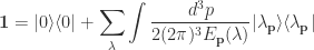
where is a general (possibly multiparticle) eigenstate of the Hamiltonian with momentum . Inserting this in the middle of the propagator we get

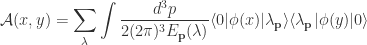
where we have assumed that the VEV vanishes, which is equivalent to no interactions at . This is a very reasonable assumption, and in fact is a key assumption for scattering processes. (It’s particularly important in the analysis of spontaneous symmetry breaking, for example).

Now a little bit of manipulation (exercise: use the transformation of the quantities under the full Poincare group) gives us that

Now substituting and introducing an integration over we get

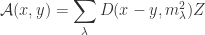
where is a Feynman propagator and 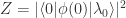is a renormalization factor. We’ll safely ignore for the rest of this post, since it doesn’t contribute to the analytic behaviour we’re interested in.

So why is this useful? One natural way to extract information from this formula might be to distinguish one-particle states. Let’s see how that helps. Recall that our states are eigenvalues of the energy-momentum operator . Generically we get one-particle states of mass arranged along a hyperboloid in energy-momentum space, due to special relativity. We also have multiparticle states of mass at least forming a continuum at higher energy and momenta. (This is obvious if you consider possible vector addition of one-particle states).

Now we can use this newfound knowledge to rewrite the sum over as an isolated one-particle term, plus an integral over the multiparticle continuum as follows

This is starting to look promising. Transforming to momentum space is the last step we need to extract something useful. We find

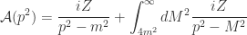
Considering the amplitude as an analytic function of the “Mandelstam variable” we find an isolated simple pole from an on-shell single particle state, plus a branch cut from multiparticle states.

It’s easy to generalize this to all Feynman diagrams. The key point is that all the analytic structure of an amplitude is encoded by the propagators. Indeed, the vertices and external legs merely contribute polarization vectors, internal symmetry factors and possibly positive factors of momentum. Singularities and branch cuts can only arise from propagators.

So what’s the big deal?

We’ve done a lot of work to extract some seemingly abstract information. But now it’s time for a substantial payoff! The analytic structure of Feynman diagrams can help us to determine their values. I won’t go into details here, but I will briefly mention one important application.

Remember that the scattering matrix in any sensible theory must conserve probabilities, and so be unitary. This requirement, coupled with our observations about Feynman diagrams tells us a lot about perturbative results. The result is usually known as the optical theorem and allows you to extract information about the discontinuities of higher loop diagrams from those at lower loops.

Still this seems rather esoteric, until you turn the whole procedure on it’s head. Suppose you are trying to guess a -loop amplitude. You know it’s general form perhaps, but need to fix some constants. Well from the -matrix unitarity we know it has a branch cut and that the discontinuity is encoded by some tree level diagrams. These diagrams are essentially given by “cutting” the loop diagram.

So go ahead and compare the discontinuity you have with the product of the relevant tree diagrams. This will give you constraints on the constants you need to fix. Do this enough times, for different “cuts” and you will have fixed your -loop amplitude. Simple!

This method is known as generalized unitarity. It’s a vital tool in the modern amplitudes box, and has been used successfully to attack many difficult loop calculations. I’ll return to it more rigorously later, and promise to show you a genuine calculation too.

Until then, enjoy your weekend!

Recursion Relations for Amplitudes

So yesterday’s discussion was all about how simple some gluon scattering processes (or amplitudes) look. In particular the maximal helicity violating (MHV) ones are special, because hundreds of terms cancel down to give a single neat result. Today I’ve been looking at how to prove this result, so I can now sketch the main ingredients for you.

If you’re from a mathsy background you won’t be surprised to learn that the -gluon Parke-Taylor identity is proved using induction. For the uninitiated there’s a simple analogy with climbing stairs. If you can get up the first one, and you can get from every one to the next one then you can get to the top!

With this in mind, our first task is to prove the simplest case, which turns out to be . Why exactly? Well the Feynman rules for QCD have 3 and 4 point vertices at tree level, so there’s no tree level 2 point amplitudes! Turns out that the case is neatly dealt with using spinor helicity formalism. Roughly speaking this takes into account the special helicity structure of the MHV amplitudes to lock in simplifications right from the start of the calculation! Add in momentum conservation and hey presto the Parke-Taylor identity drops right out.

So now we need to climb from one stair to the next. This is where recursion relations come in handy. Nine years ago, a group of theoreticians spotted a cunning way to break apart tree level gluon amplitudes into smaller, more manageable pieces. Mathematically they spotted that the -gluon scattering amplitude factorized into the product of two distinct on-shell amplitudes, each with a complementary subset of the original external legs plus an extra leg with momentum . The only added ingredient needed was a factor of corresponding to a propagator between the two diagrams.

Woah – hold up there! What’s all this terminology all of a sudden. For the uninitiated I’m guessing that on-shell sounds a bit confusing. But it’s no cause for alarm. In general an on-shell quantity is one which obeys the equations of motion of the system involved. Here the relevant equation is the Weyl equation, which implies that .

Why are these recursion relations so useful? Well, they give us exactly the ingredient we needed for the induction step. And we’re done – the Parke-Taylor identity is proved, with a little bit of algebra I’ve shoved under the rug.

There’s one more point I’ve neglected to mention. How do you go about finding these mythical on-shell recursion relations? The answer comes from doing some subtle complex analysis, transforming momenta into the complex plane. It might not sound very physical to do that, but in fact the method opens up oodles of new possibilities. One reason is that complex integration is both more powerful and easier than its real counterpart, so it can be used to extract valuable identities from the world of scattering processes.

I’ll leave you with this great basic article clarifying the subtleties of the on-shell/off-shell distinction. It goes a bit deeper than that too, so is worth a read even if you’re more of an expert!

Tomorrow I hope I’ll bring you something more supersymmetrical in nature. SUSY is a favourite playground for scattering enthusiasts because it is finite (no renormalization needed) and very simple (no free parameters). We’ll encounter its stark beauty in due course.

The Parke-Taylor Formula

Unfortunately I’m not going to have time today to give you a full post, mostly due to an abortive mission to Barking! The completion of that mission tomorrow may impact on post length again, so stay tuned for the first full PhD installment.

Nonetheless, here’s a brief tidbit from my first day. Let’s think about the theory of the strong force, which binds quarks and nuclei together. Mathematically it’s governed by quantum chromodynamics (QCD). At it’s simplest we can study QCD with no matter, so just consider the scattering interactions of the force carrying gluon particles.

It turns out that even this is pretty complicated! At tree level in Feynman diagram calculations, the simplest possible approximation, there are about 12000 terms for a four gluon scattering event. Thankfully these all cancel to give a single, closed form expression for the scattering amplitude. But why?

There’s a simpler way that makes use of some clever tricks to prove the more general Parke-Taylor formula that the maximal helicity violating gluon amplitude is simply

What does this all mean?

Qualitatively, that there is a formalism in which these calculations come out very simply and naturally. This will be the starting point for my exploration of modern day amplitudology – a subject that ranges through twistor theory, complex analysis and high dimensional geometry!

For the real mathematics behind the formula above, I’m afraid you’ll have to wait until tomorrow or Wednesday!